See the follow up post where I introduce my R package and spreadsheet TOSTER to perform TOST equivalence tests, and link to a practical primer on this topic.
When you find p > 0.05, you did not observe surprising data, assuming there is no true effect. You can often read in the literature how p > 0.05 is interpreted as ‘no effect’ but due to a lack of power the data might not be surprising if there was an effect. In this blog I’ll explain how to test for equivalence, or the lack of a meaningful effect, using equivalence hypothesis testing. I’ve created easy to use R functions that allow you to perform equivalence hypothesis tests. Warning: If you read beyond this paragraph, you will never again be able to write “as predicted, the interaction revealed there was an effect for participants in the experimental condition (p < 0.05) but there was no effect in the control condition (F < 1).” If you prefer the veil of ignorance, here’s a nice site with cute baby animals to spend the next 9 minutes on instead.
When you find p > 0.05, you did not observe surprising data, assuming there is no true effect. You can often read in the literature how p > 0.05 is interpreted as ‘no effect’ but due to a lack of power the data might not be surprising if there was an effect. In this blog I’ll explain how to test for equivalence, or the lack of a meaningful effect, using equivalence hypothesis testing. I’ve created easy to use R functions that allow you to perform equivalence hypothesis tests. Warning: If you read beyond this paragraph, you will never again be able to write “as predicted, the interaction revealed there was an effect for participants in the experimental condition (p < 0.05) but there was no effect in the control condition (F < 1).” If you prefer the veil of ignorance, here’s a nice site with cute baby animals to spend the next 9 minutes on instead.
Any science that wants to be taken seriously needs to be
able to provide support for the null-hypothesis. I often see people switching
over from Frequentist statistics when effects are significant, to the use of
Bayes Factors to be able to provide support for the null hypothesis. But it is
possible to test if there is a lack of an effect using p-values (why no one ever told me this in the 11 years I worked in science is beyond me). It’s as easy as doing a
t-test, or more precisely, as doing two t-tests.
The practice of Equivalence Hypothesis Testing (EHT) is used
in medicine, for example to test whether a new cheaper drug isn’t worse (or
better) than the existing more expensive option. A very simple EHT approach is the
‘two-one-sided t-tests’ (TOST)
procedure (Schuirmann,
1987).
Its simplicity makes it wonderfully easy to use.
The basic idea of the test is to flip things around: In
Equivalence Hypothesis Testing the null hypothesis is that there is a true
effect larger than a Smallest Effect Size of Interest (SESOI; Lakens,
2014).
That’s right – the null-hypothesis is now that there IS an effect, and we are
going to try to reject it (with a p < 0.05). The alternative hypothesis is
that the effect is smaller than a SESOI, anywhere in the equivalence range - any effect you think is too small to matter, or too small to feasibly examine. For example, a Cohen’s d of 0.5 is a medium
effect, so you might set d = 0.5 as your SESOI, and the equivalence range goes
from d = -0.5 to d = 0.5 In the TOST procedure, you first decide upon your
SESOI: anything smaller than your smallest effect size of interest is
considered smaller than small, and will allow you to reject the null-hypothesis
that there is a true effect. You perform two t-tests, one testing if the effect is smaller than the upper bound
of the equivalence range, and one testing whether the effect is larger than the
lower bound of the equivalence range. Yes, it’s that simple.
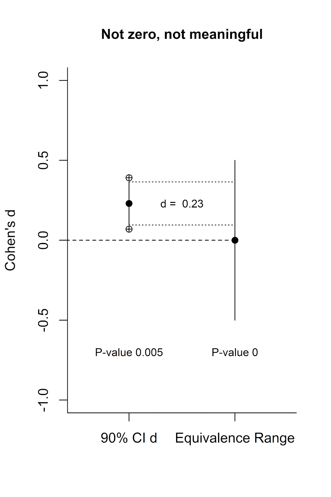
Let’s visualize this. Below on the left axis is a scale for
the effect size measure Cohen’s d. On the left is a single 90% confidence
interval (the crossed circles indicate the endpoints of the 95% confidence
interval) with an effect size of d = 0.13. On the right is the equivalence
range. It is centered on 0, and ranges from d = -0.5 to d = 0.5.

We see from the 95% confidence interval around d = 0.13 (again,
the endpoints of which are indicated by the crossed circles) that the lower
bound overlaps with 0. This means the effect (d = 0.13, from an independent t-test with two conditions of 90
participants each) is not statistically different from 0 at an alpha of 5%, and
the p-value of the normal NHST is
0.384 (the title provides the exact numbers for the 95% CI around the effect
size). But is this effect statistically smaller than my smallest effect size of
interest?
Rejecting the presence of a meaningful effect
There are two ways to test the lack of a meaningful effect
that yield the same result. The first is to perform two one sided t-tests,
testing the observed effect size against the ‘null’ of your SESOI (0.5 and
-0.5). These t-tests show the d = 0.13 is significantly larger than d = -0.5,
and significantly smaller than d = 0.5. The highest of these two p-values is p = 0.007. We can conclude that there is support for the lack of a
meaningful effect (where meaningful is defined by your choice of the SESOI).
The second approach (which is easier to visualize) is to calculate a 90% CI
around the effect (indicated by the vertical line in the figure), and check whether this 90% CI
falls completely within the equivalence range. You can see a line from the
upper and lower limit of the 90% CI around d = 0.13 on the left to the
equivalence range on the right, and the 90% CI is completely contained within
the equivalence range. This means we can reject the null of an effect that is
larger than d = 0.5 or smaller than d = -0.5 and conclude this effect is
smaller than what we find meaningful (and you’ll be right 95% of the time, in
the long run).
[Technical note: The reason we are using a 90% confidence
interval, and not a 95% confidence interval, is because the two one-sided tests
are completely dependent. You could actually just perform one test, if the
effect size is positive against the upper bound of the equivalence range, and
if the effect size is negative against the lower bound of the equivalence
range. If this one test is significant, so is the other. Therefore, we can use
a 90% confidence interval, even though we perform two one-sided tests. This is also why
the crossed circles are used to mark the 95% CI.].
So why were we not using these tests in the psychological
literature? It’s the same old, same old. Your statistics teacher didn’t tell
you about them. SPSS doesn’t allow you to do an equivalence test. Your editors
and reviewers were always OK with your statements such as “as predicted, the
interaction revealed there was an effect for participants in the experimental
condition (p < 0.05) but there was no effect in the control condition (F
< 1).” Well, I just ruined that for you. Absence of evidence is not evidence
of absence!
We can’t use p > 0.05 as evidence of a lack of an effect.
You can switch to Bayesian statistics if you want to support the null, but the
default priors are only useful of in research areas where very large effects
are examined (e.g., some areas of cognitive psychology), and are not
appropriate for most other areas in psychology, so you will have to be able to
quantify your prior belief yourself. You can teach yourself how, but there
might be researchers who prefer to provide support for the lack of an effect
within a Frequentist framework. Given that most people think about the effect
size they expect when designing their study, defining the SESOI at this moment
is straightforward. After choosing the SESOI, you can even design your study to
have sufficient power to reject the presence of a meaningful effect.
Controlling your error rates is thus straightforward in equivalence hypothesis
tests, while it is not that easy in Bayesian statistics (although it can be
done through simulations).
One thing I noticed while reading this literature is that
TOST procedures, and power analyses for TOST, are not created to match the way
psychologists design studies and think about meaningful effects. In medicine,
equivalence is based on the raw data (a decrease of 10% compared to the default
medicine), while we are more used to think in terms of standardized effect
sizes (correlations or Cohen’s d). Biostatisticians are fine with estimating
the pooled standard deviation for a future study when performing power analysis
for TOST, but psychologists use standardized effect sizes to perform power
analyses. Finally, the packages that exist in R (e.g., equivalence) or the
software that does equivalence hypothesis tests (e.g., Minitab, which has TOST
for t-tests, but not correlations)
requires that you use the raw data. In my experience (Lakens,
2013)
researchers find it easier to use their own preferred software to handle their data, and then
calculate additional statistics not provided by the software they use by typing
in summary statistics in a spreadsheet (means, standard deviations, and sample
sizes per condition). So my functions don’t require access to the raw data
(which is good for reviewers as well). Finally, the functions make a nice
picture such as the one above so you can see what you are doing.
R Functions
I created R functions for TOST for independent t-tests, paired samples t-tests, and correlations, where you can
set the equivalence thresholds using Cohen’s d, Cohen’s dz, and r. I adapted
the equation for power analysis to be based on d, and I created the equation
for power analyses for a paired-sample t-test from scratch because I couldn’t
find it in the literature. If it is not obvious: None of this is peer-reviewed
(yet), and you should use it at your own risk. I checked the independent andpaired t-test formulas against theresults from Minitab software and reproduced examples in the literature, and checked the power analyses against simulations, and all yielded the expected results, so that’s comforting. On the other
hand, I had never heard of equivalence testing until 9 days ago (thanks 'Bum Deggy'), so that’s less
comforting I guess. Send me an email if you want to use these formulas for anything serious
like a publication. If you find a mistake or misbehaving functions, let me
know.
If you load (select and run) the functions (see GitHub gist below), you can perform a TOST by entering the correct numbers and running the single line of
code:
TOSTd(d=0.13,n1=90,n2=90,eqbound_d=0.5)
You don’t know how to calculate Cohen’s d in an independent
t-test? No problem. Use the means and standard deviations in each group
instead, and type:
TOST(m1=0.26,m2=0.0,sd1=2,sd2=2,n1=90,n2=90,eqbound_d=0.5)
You’ll get the figure above, and it calculates Cohen’s d and
the 95% CI around the effect size for free. You are welcome. Note that TOST and
TOSTd differ slightly (TOST relies on the t-distribution, TOSTd on the
z-distribution). If possible, use TOST – but TOSTd (and especially TOSTdpaired)
will be very useful for readers of the scientific literature who want quickly
check the claim that there is a lack of effect when means or standard
deviations are not available. If you prefer to set the equivalence in raw
difference scores (e.g., 10% of the mean in the control condition, as is common
in medicine) you can use the TOSTraw function.
Are you wondering if your design was well powered? Or do you
want to design a study well-powered to reject a meaningful effect? No problem.
For an alpha (Type 1 error rate) of 0.05, 80% power (or a beta or Type 2 error
rate of 0.2), and a SESOI of 0.4, just type:
powerTOST(alpha=0.05, beta=0.2, eqbound_d=0.4) #Returns n
(for each condition)
You will see you need 107 participants in each condition to
have 80% power to reject an effect larger than d = 0.4, and accept the null (or
an effect smaller than your smallest effect size of interest). Note that this
function is based on the z-distribution, it does not use the iterative approach
based on the t-distribution that would make it exact – so it is an
approximation but should work well enough in practice.
TOSTr will perform these calculations for correlations, and
TOSTdpaired will allow you to use Cohen’s dz to perform these calculations for
within designs. powerTOSTpaired can be used when designing within subject
design studies well-powered to test if data is in line with the lack of a
meaningful effect.
Choosing your SESOI
How should you choose your SESOI? Let me quote myself
(Lakens, 2014, p. 707):
In applied research,
practical limitations of the SESOI can often be determined on the basis of a
cost–benefit analysis. For example, if an intervention costs more money than it
saves, the effect size is too small to be of practical significance. In
theoretical research, the SESOI might be determined by a theoretical model that
is detailed enough to make falsifiable predictions about the hypothesized size
of effects. Such theoretical models are rare, and therefore, researchers often
state that they are interested in any effect size that is reliably different
from zero. Even so, because you can only reliably examine an effect that your
study is adequately powered to observe, researchers are always limited by the
practical limitation of the number of participants that are willing to
participate in their experiment or the number of observations they have the
resources to collect.
Let’s say you collect 50 participants in two independent
conditions, and plan to do a t-test
with an alpha of 0.05. You have 80% power to detect an effect with a Cohen’s d
of 0.57. To have 80% power to reject an effect of d = 0.57 or larger in TOST
you would need 66 participants in each condition.
Let’s say your SESOI is actually d = 0.35. To have 80% power
in TOST you would need 169 participants in each condition (you’d need 130
participants in each condition to have 80% power to reject the null of d = 0 in
NHST).
Conclusion
We see you always need a bit more people to reject a
meaningful effect, than to reject the null for the same meaningful effect.
Remember that since TOST can be performed based on Cohen’s d, you can use it in
meta-analyses as well (Rogers,
Howard, & Vessey, 1993). This is a great place to use
EHT and reject a small effect (e.g., d = 0.2, or even d = 0.1), for which you
need quite a lot of observations (i.e., 517, or even 2069).
Equivalence testing has many benefits. It fixes the
dichotomous nature of NHST. You can now 1) reject the null, and fail to reject
the null of equivalence (there is probably something, of the size you find
meaningful), 2) reject the null, and reject the null of equivalence (there is
something, but it is not large enough to be meaningful, 3) fail to reject the
null, and reject the null of equivalence (the effect is smaller than anything
you find meaningful), and 4) fail to reject the null, and fail to reject the
null of equivalence (undetermined: you don’t have enough data to say there is
an effect, and you don’t have enough data to say there is a lack of a
meaningful effect). These four situations are visualized below.
There are several papers throughout the scientific
disciplines telling us to use equivalence testing. I’m definitely not the
first. But in my experience, the trick to get people to use better statistical
approaches is to make it easy to do so. I’ll work on a manuscript that tries to make these tests easy to use (if you read this post this far, and work for a journal that might be
interested in this, drop me a line – I’ll throw in an easy to use spreadsheet just
for you). Thinking about meaningful effects in terms of standardized effect
sizes and being able to perform these test based on summary statistics might
just do the trick. Try it.


Lakens, D.
(2013). Calculating and reporting effect sizes to facilitate cumulative
science: a practical primer for t-tests and ANOVAs. Frontiers in Psychology,
4. http://doi.org/10.3389/fpsyg.2013.00863
Lakens, D. (2014). Performing high-powered studies efficiently with
sequential analyses: Sequential analyses. European Journal of Social
Psychology, 44(7), 701–710. http://doi.org/10.1002/ejsp.2023
Rogers, J. L., Howard, K. I., & Vessey, J. T. (1993). Using
significance tests to evaluate equivalence between two experimental groups. Psychological
Bulletin, 113(3), 553.
Schuirmann, D. J. (1987). A comparison of the two one-sided tests
procedure and the power approach for assessing the equivalence of average bioavailability.
Journal of Pharmacokinetics and Biopharmaceutics, 15(6), 657–680.
The R-code that was part of this blog post is temporarily unavailable as I move it to a formal R package.